Source:
References: http://theory.stanford.edu/~amitp/GameProgramming/
00:01
Welcome to this video on pathfinding. So in this first episode, we’re going to be taking a look at how the A* algorithm actually works so that once we begin programming it in the future episodes, you’ve got a pretty good understanding of why it works and where we’re going.
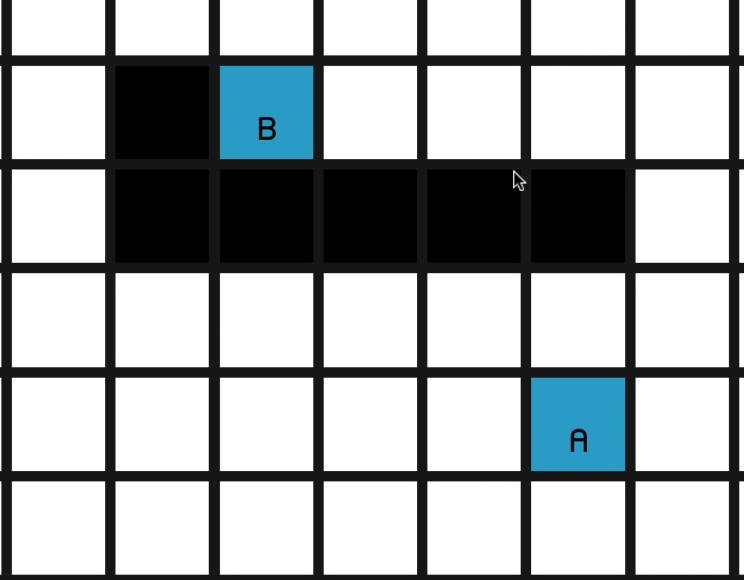
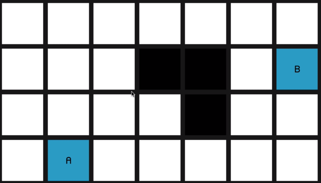
All right, so here we have a grid of nodes,

the white nodes representing the walkable areas in our map and the black nodes representing the obstacles.
00:32
So of course we’re trying to find the shortest path from node A to node B, and what we need to do first is decide how far apart the nodes are. So it would be quite natural to say that the distance between two nodes is one. And therefore, by Pythagoras, the distance diagonally is going to be the square root of two, which is approximately one point four. So quite a common practice is just to multiply those two numbers by 10
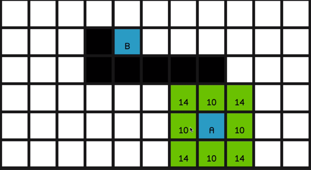
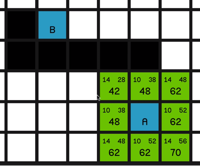
and to use 01:00 the nice integer values of 10 across and vertically and 14 for the diagonals. All right. So I’ll remove the obstacles for a moment so we can see how the algorithm is going to run when there aren’t any obstructions. So the algorithm begins by going to the starting node, node A over here, and looking at all of its surrounding nodes
and calculating some values for each of them.
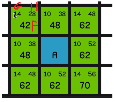
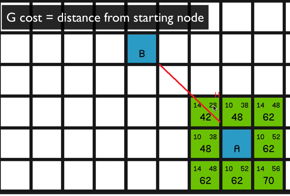
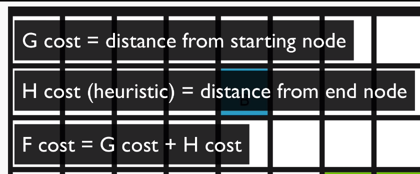
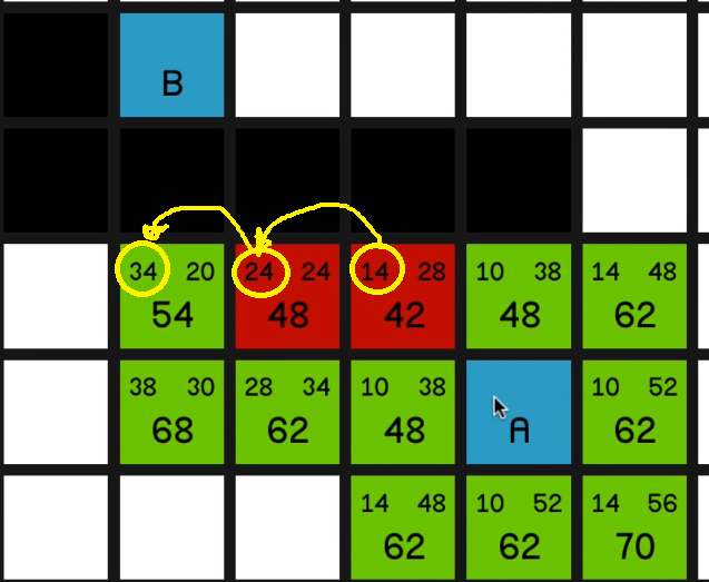
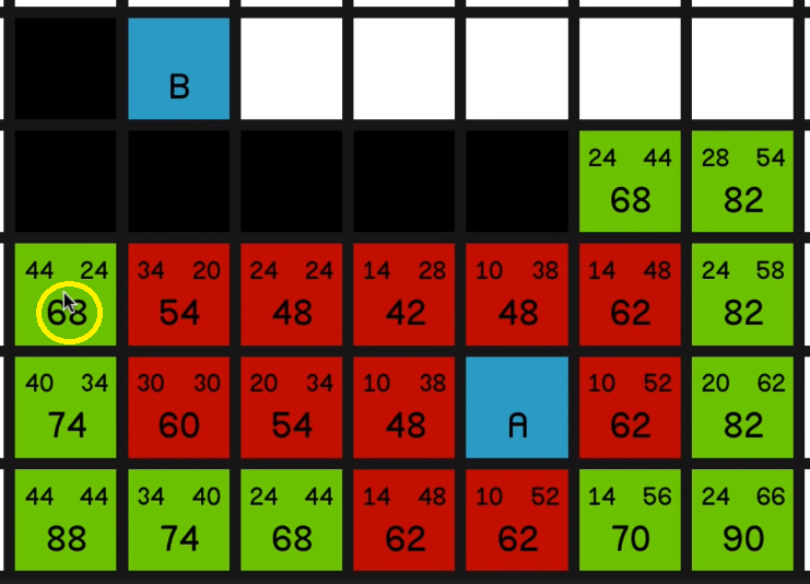
So the values in the top left corner of each node are called the nodes G cost.
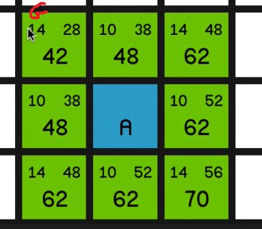
And that is quite simply how far away that node is from the starting node. So this node in the top left corner has got a
G cost of 14 since it’s just one diagonal move away from node A.
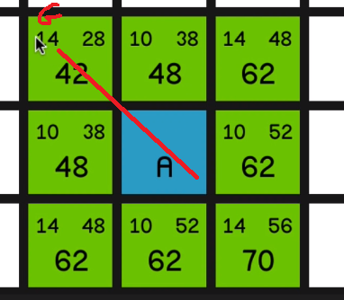
In the top right corner of each node is the nodes H cost, which is basically the opposite of G cost. It’s how far away the node is from the end node. So this node is two diagonal moves away from the end node so it’s got a H cost of 28.
01:58
Now the big number is the nodes’ F cost, and that is very simply G cost plus H cost.
So now the algorithm is going to look at all of these nodes and it’s going to choose the one with the lowest F cost to look at first. And that is, of course, this 42 in the top left corner.
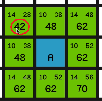
So it will mark this now as closed, so it will appear red,
and it will then calculate all of 02:31 these values again for all of its surrounding nodes.

And it’s quite simple to see what’s happening here. These F costs are just staying the same as it
moves towards the target,
because the G costs (the movement costs) are increasing
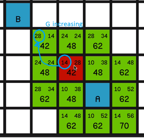
and the H costs are decreasing and they’re just sort of balancing each other out.
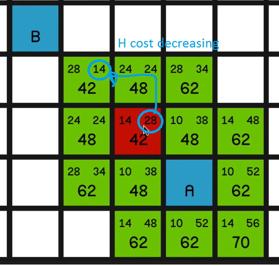
So it basically explores the path straight to the end.
02:57
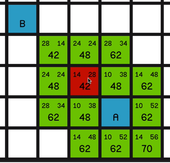
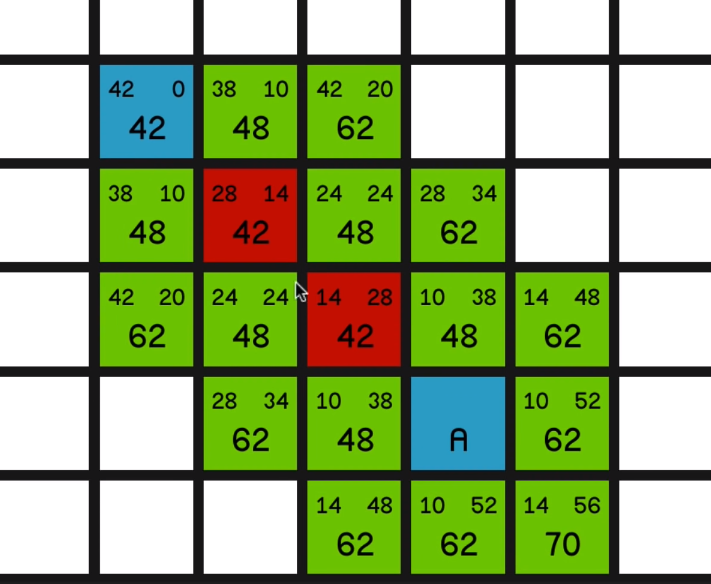
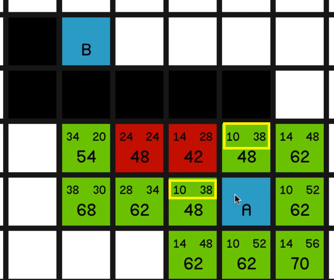
Well, no point having pathfinding in your game if you’re not going to have any obstacles. So let’s add those back in and run through the algorithm once more and see what happens.
So once again, we look at all of the surrounding nodes and calculate the F costs,
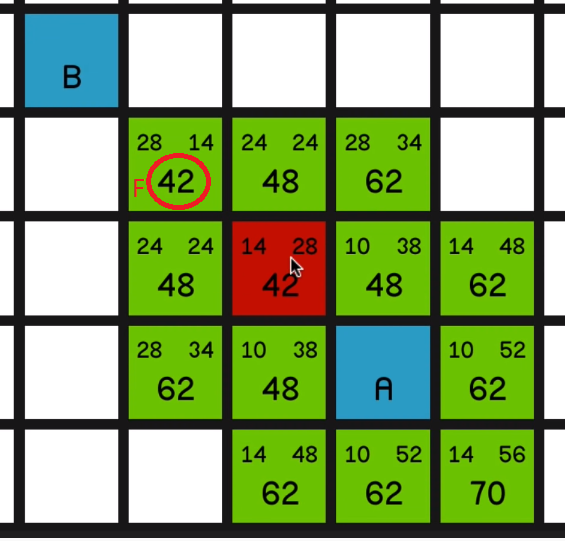
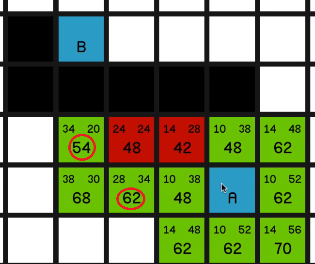
and we’ll go with this lowest F cost of 42. And now we have a scenario where we have
three nodes each with an equal F cost of 48.
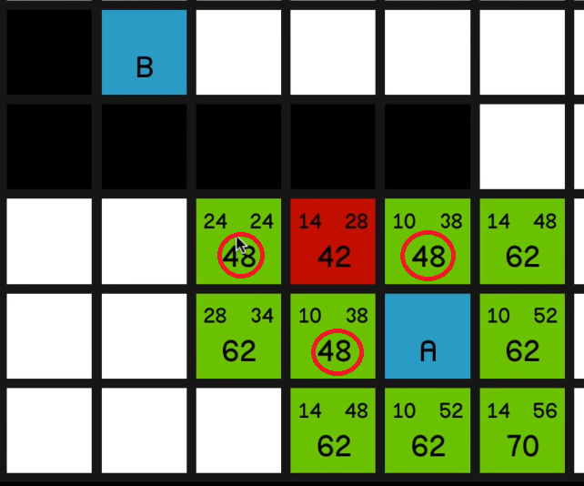
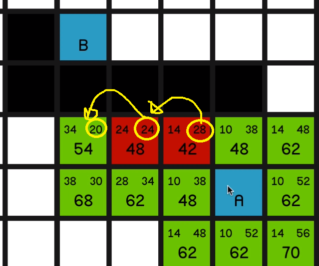
And so what we’ll do to decide which one to pick is 03:26 we’ll look at which one is closest to the
end node. In other words, which one has the lowest H cost.
This has an H cost of 38, this is also 38, and this one is 24 so we’ll go with this one.
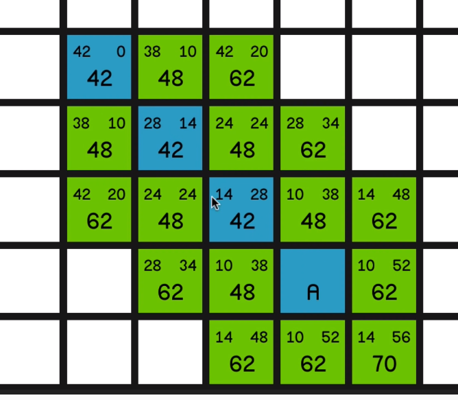
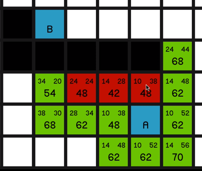
Now, as you can see, the F costs are increasing each time since we’re not going in a straight line towards
the end.
So even though the H costs are decreasing by a little bit each time,
the G costs are increasing by even more, resulting in a more expensive path.
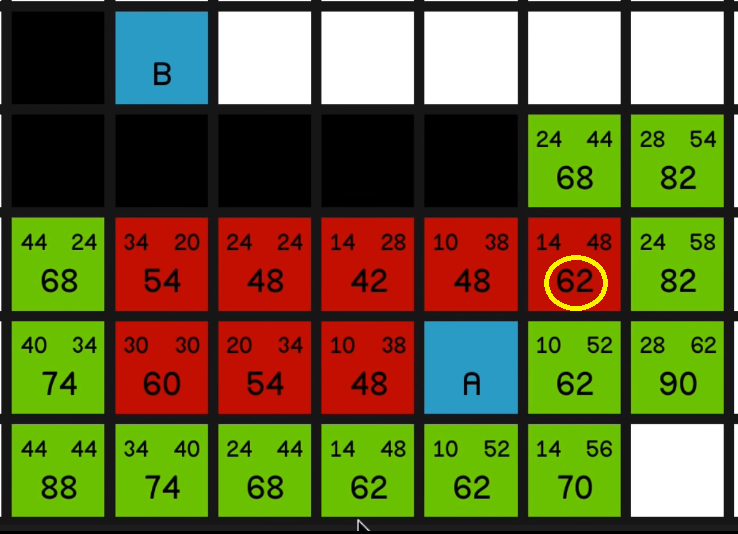
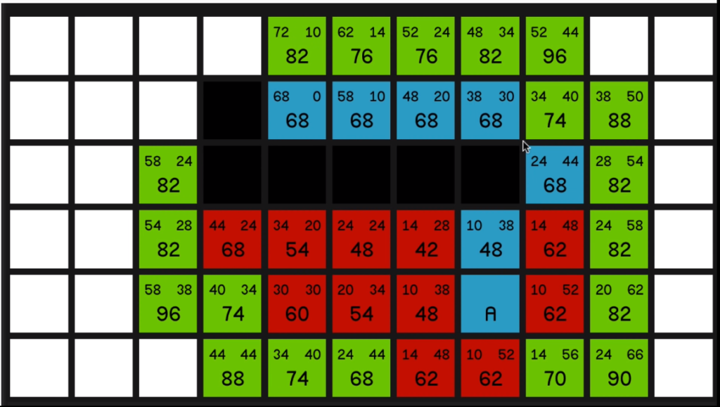
So now the two nodes with the lowest F cost on the map are these two “48”s over here.
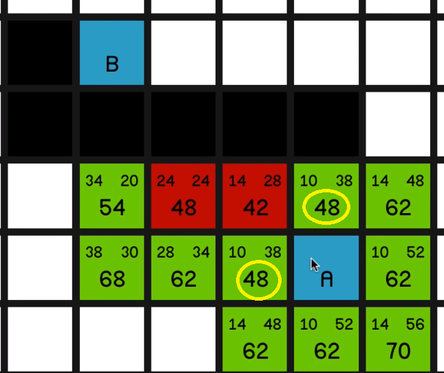
They’ve got the same H costs, so we can pretty much choose one at random.
Let’s go for this one over here… and now we have to look at the other one.
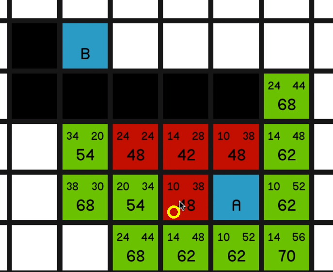
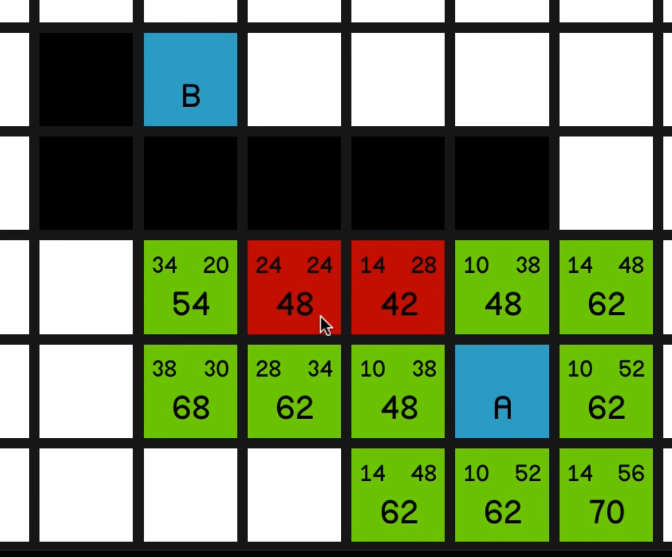
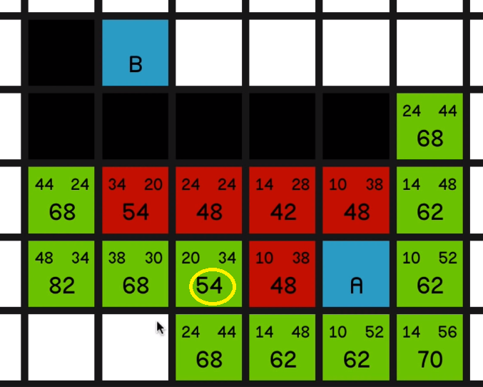
And at this point, the most sort of promising node is the 54 over here.
04:18 And we explore that… So now we’ll look at this other node with an F cost of 54.
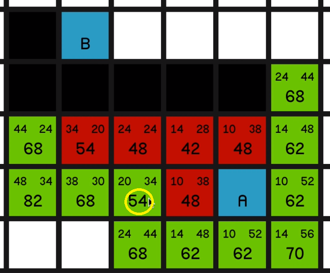
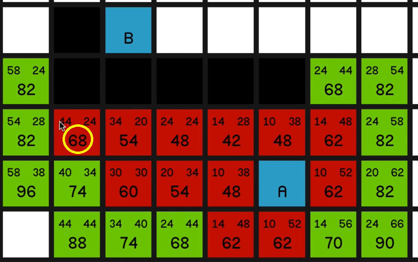
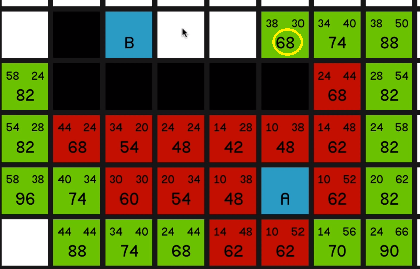
But one thing I would like to draw your attention to quickly is the node just to the left of it with an F cost of 68.
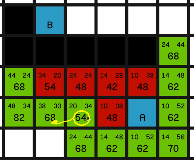
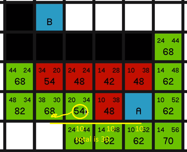
If we look at its G cost, it is currently 38. But if we look how far away it is actually from node A, it’s just 10, 20, 30 away.
04:41
So obviously this has come on the path, something like diagonally up here, 14, then across for 24 and then down diagonally to make 38.
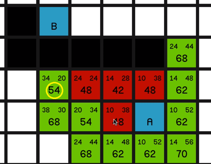
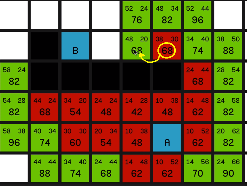
So as we explore this 54 over here
and explore all of its surrounding nodes, you’ll see how the 68 updates to reflect the new best path to this node.
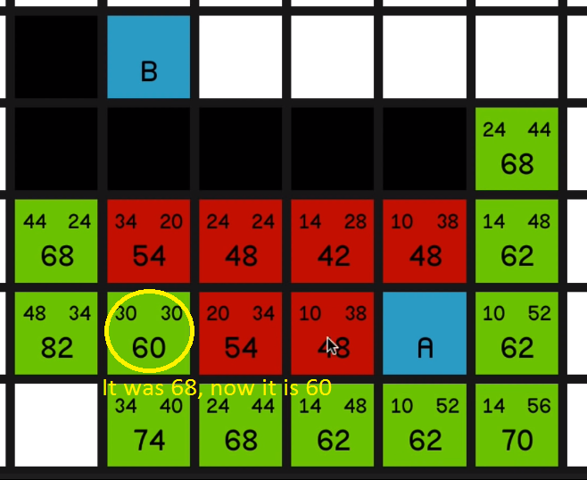
So it now has an F cost of 60 and it is the most promising node on the map. So we’ll explore that. 05:16
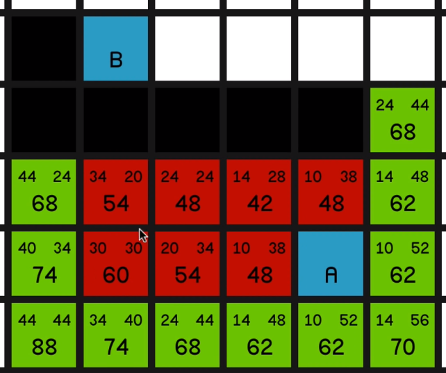
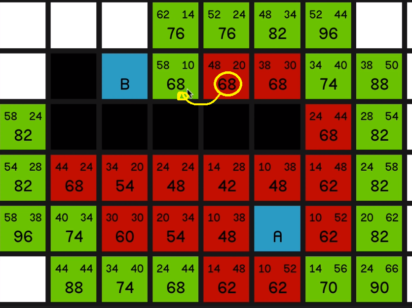
And now we have a bunch of 62s to look at.
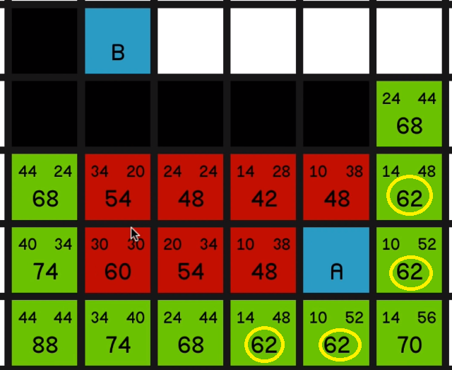
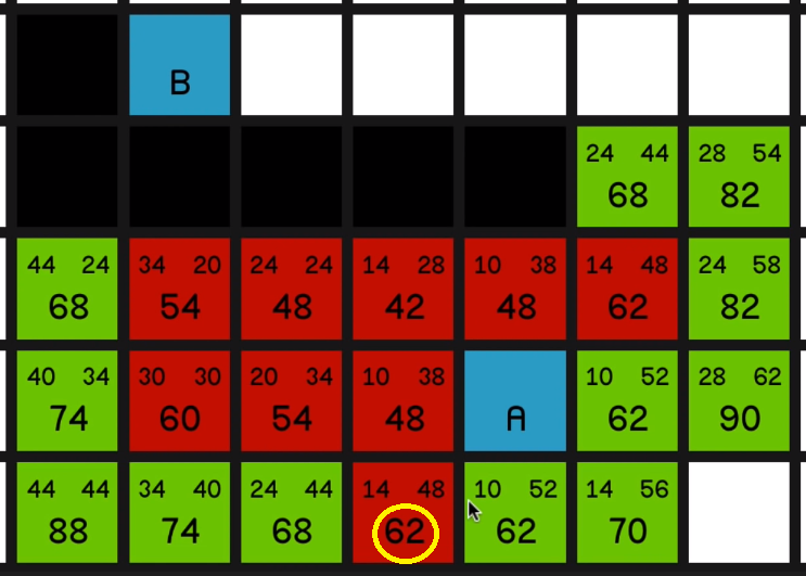
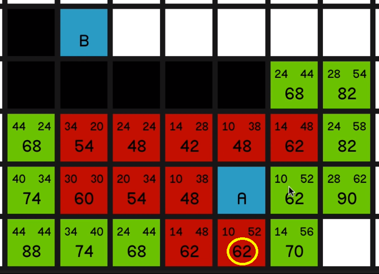
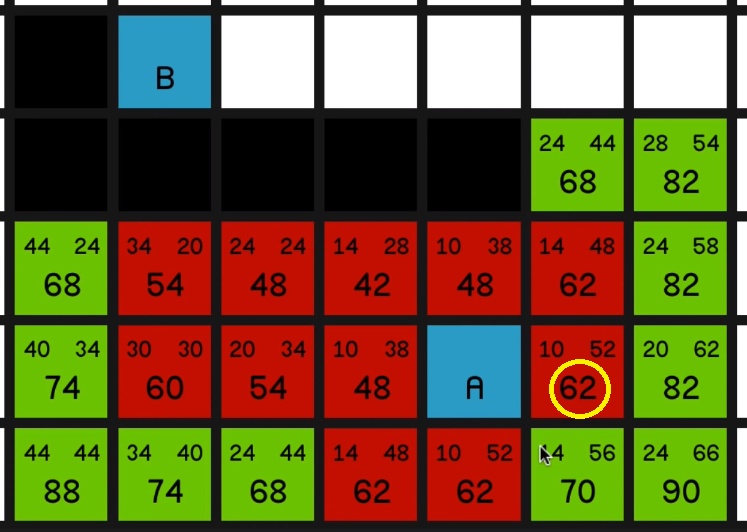
Not much say in the way of commentary here. Just exploring all of these lowest F costs until
now we can come back to the 68 and we explore that
and we get to explore the other 68
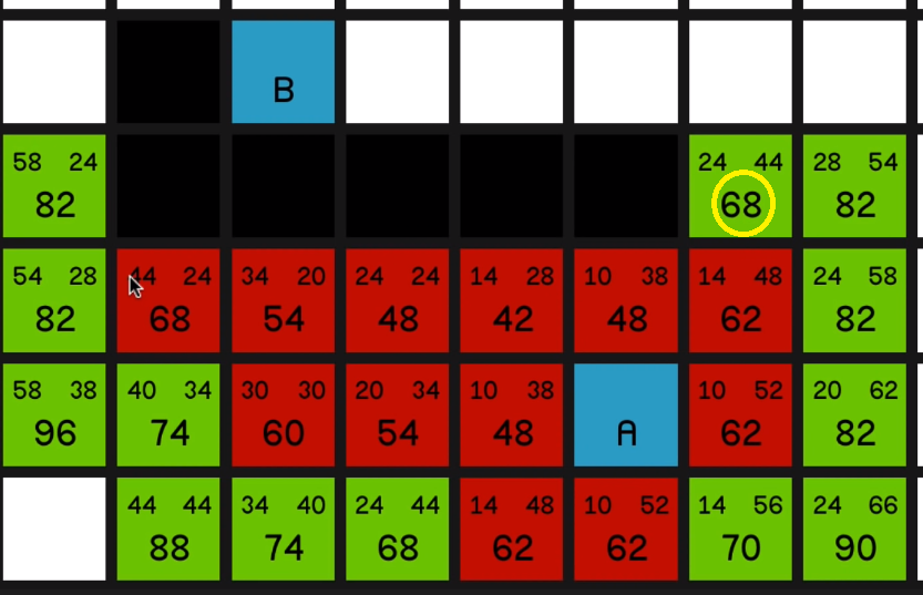
and now we’ll observe the same effect that we saw in the first example where we’ve just got a straight line to the end node and the G costs and the H costs 05:44 are going to balance each other out and the F costs won’t change, and we just go straight to the end.
So hopefully you can see how this is guaranteed to find the shortest path since as soon as you’re not moving in a straight line towards the end, the F costs are going to increase and then it will start looking at the other potential options.
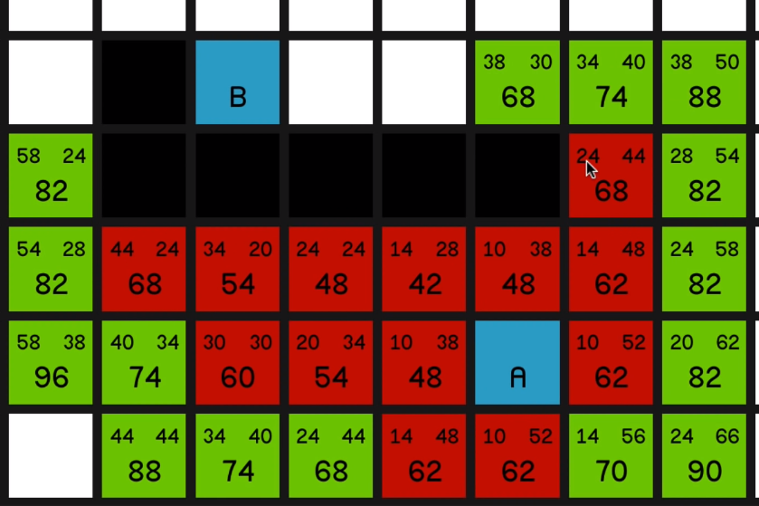
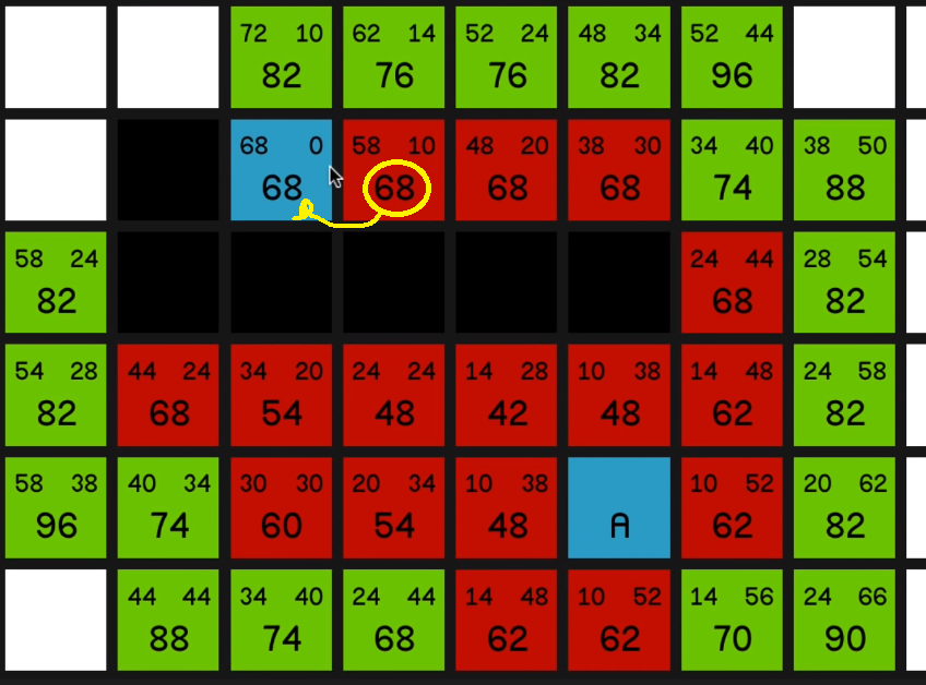
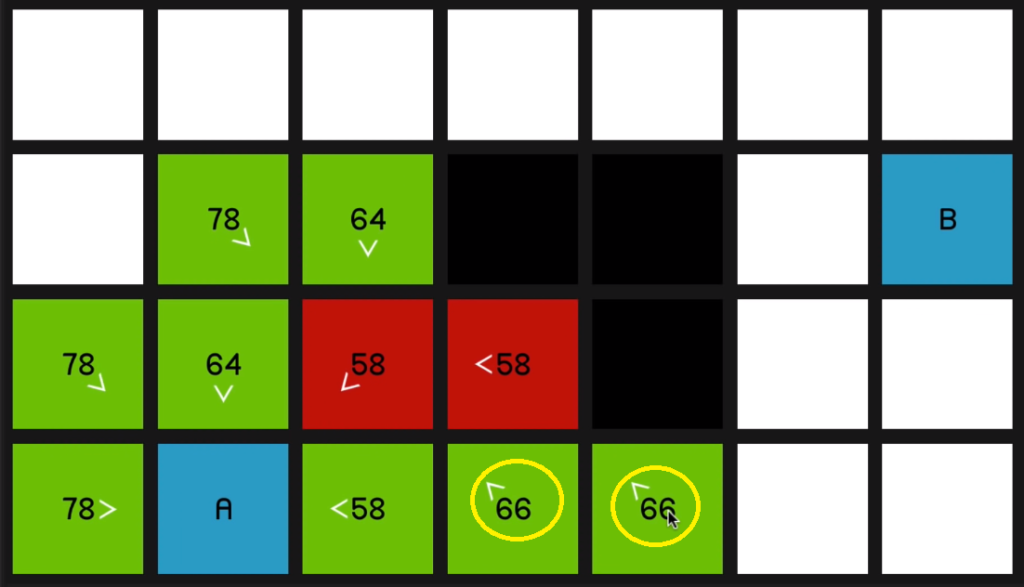
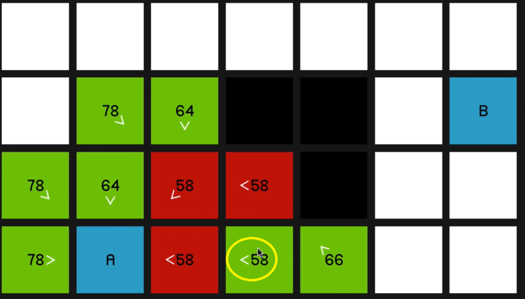
Let’s look at one final example.
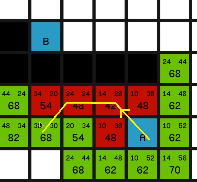
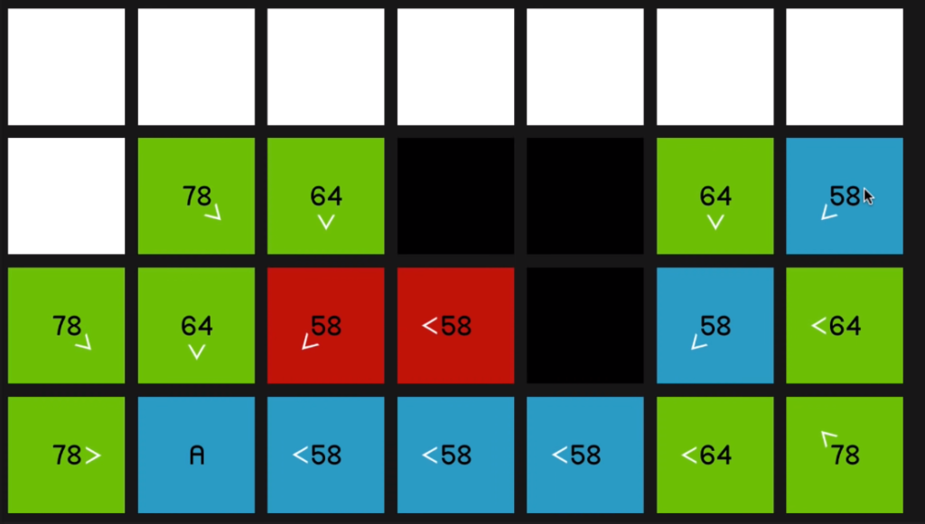
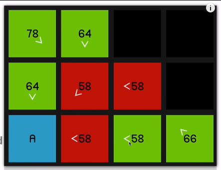
In this case, I have hidden the G costs and the H costs, and I’m instead showing these 06:15
little arrow which are basically indicating where these nodes have come from.
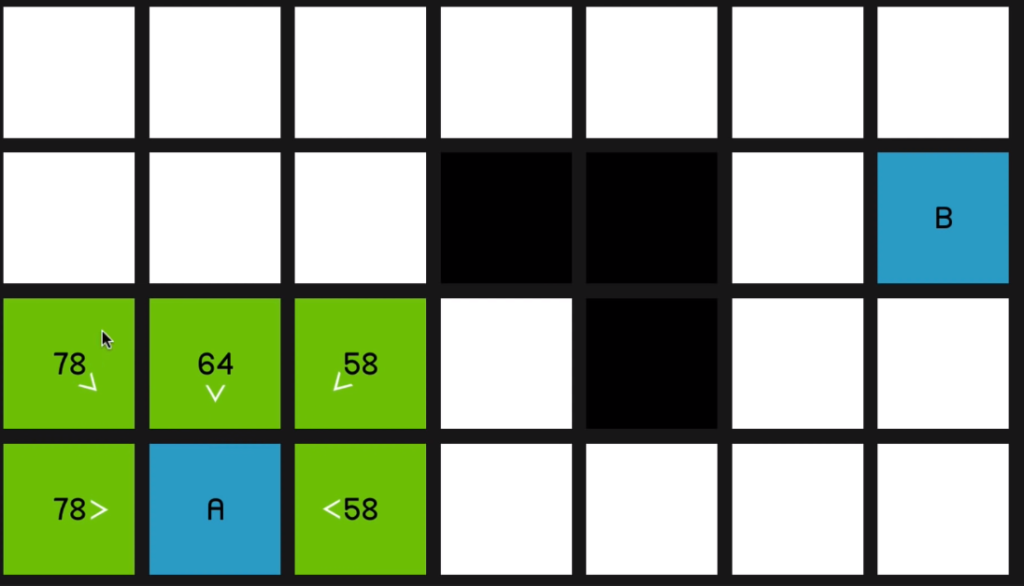
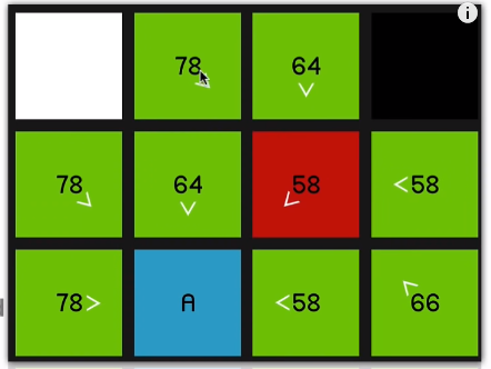
So when we explore this 58 over here,
you can see all of its surrounding nodes are now pointing to reflect that they sort of originated from this node.
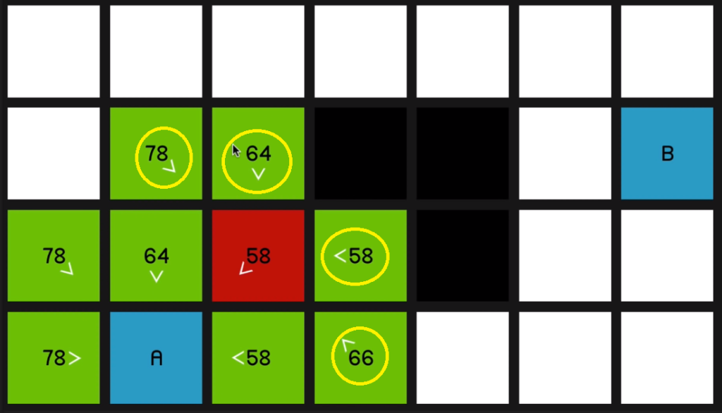
Of course, the 64 and this 58 over here,
even though they are its neighbors (neighbours of the red 58) they have not updated to to show that they’re coming from the red 58 node since it should then be a worse path. In other words, it would have a higher F cost
if we were to get to, say, this node over 06:46 here by going diagonally up and then down.
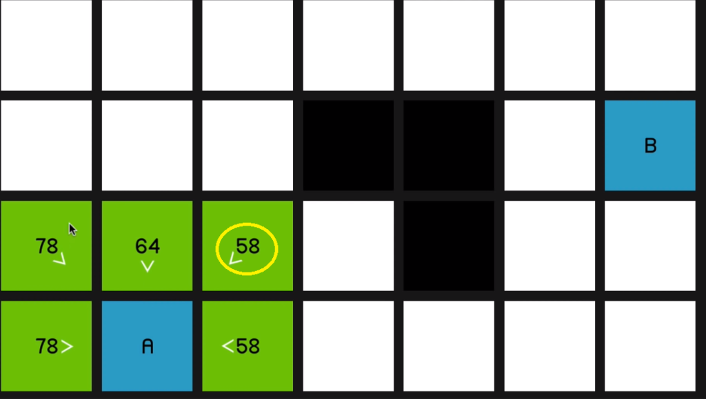
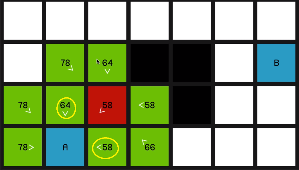
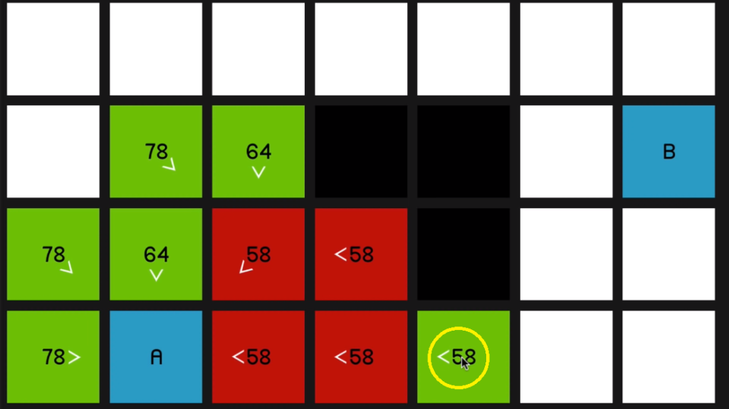
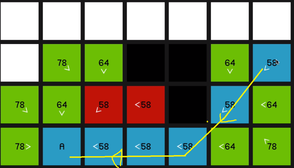
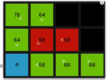
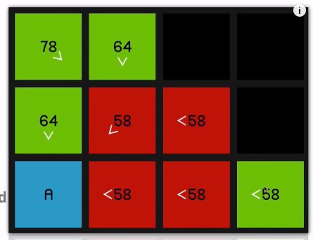
So it’ll only update if it is, in fact a better path that’s being offered. So we continue by looking at this 58
and that yields a 66.
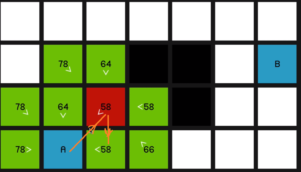
So we go back to the 58 at the beginning. And now once again, just to demonstrate 66 is coming on the sort of slower diagonal path.
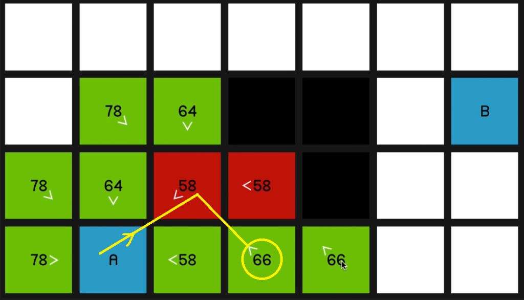
07:09 So it will be much quicker to just go horizontally across.
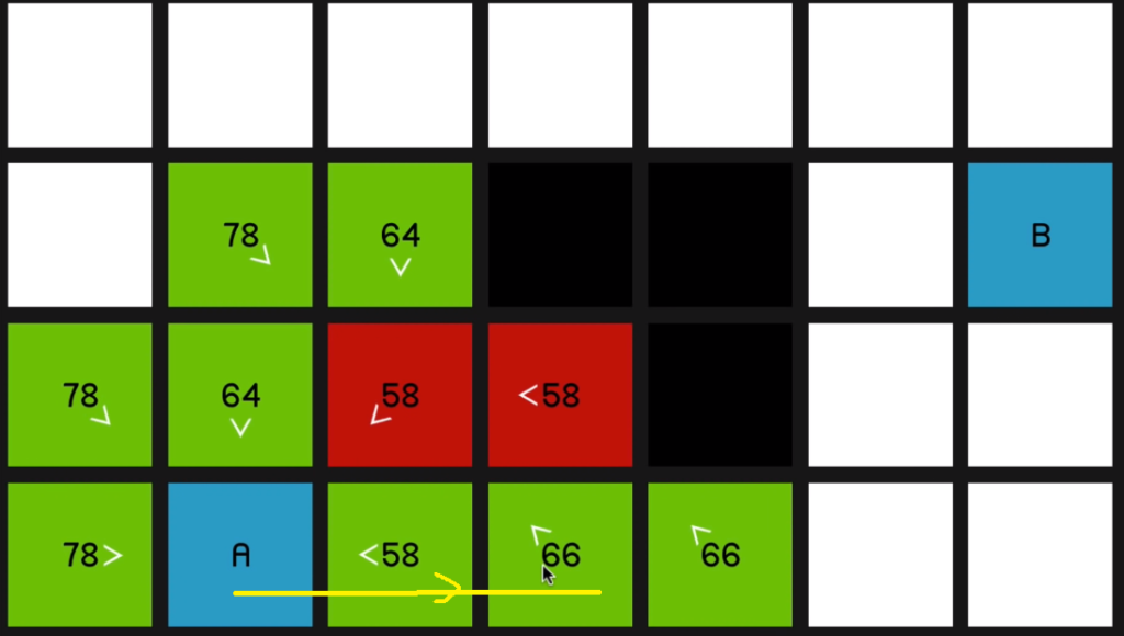
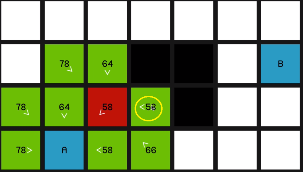
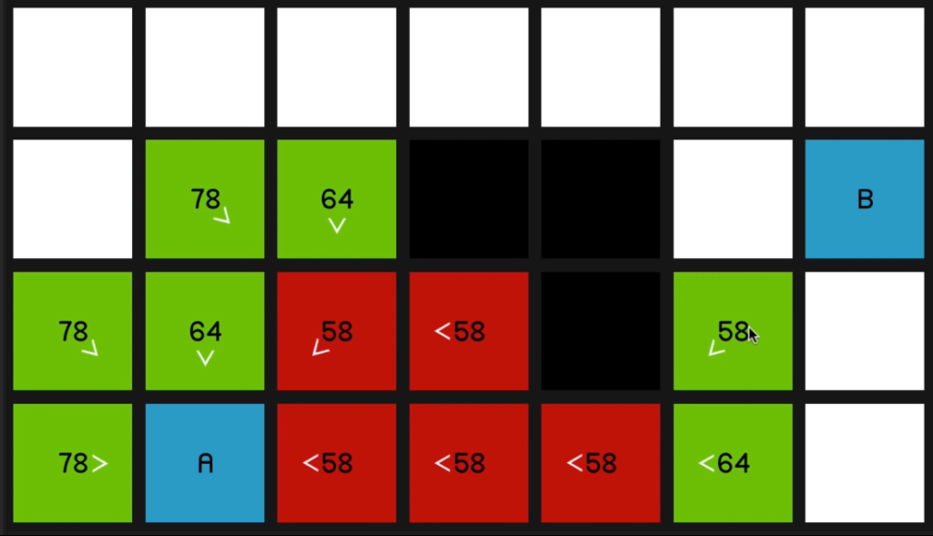
So as we explore this 58
and look at all of its surrounding nodes,
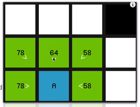
that node is going to update to reflect that.
And as you can imagine, we just go straight to the end now.
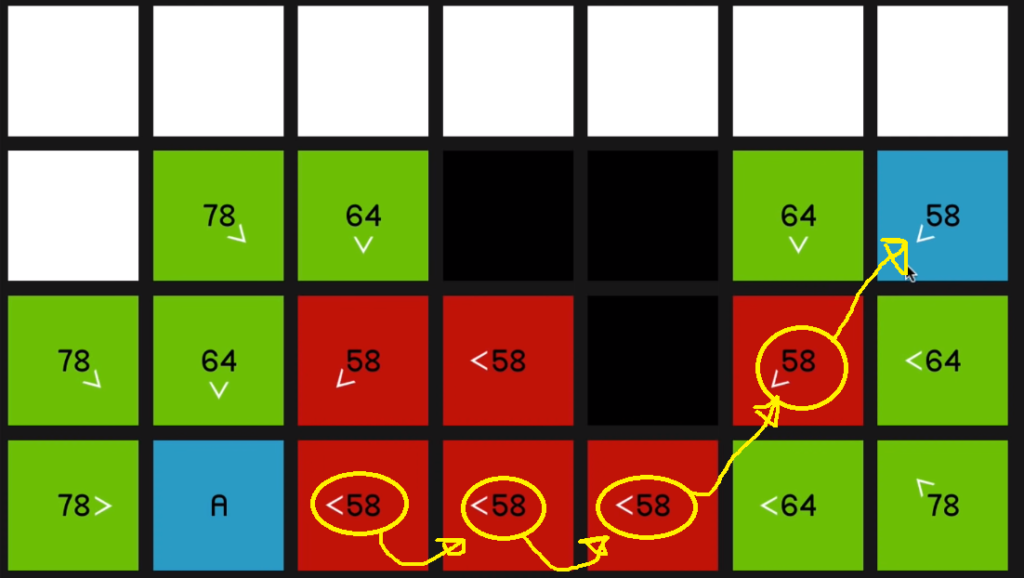
So the point of these arrows, of course, is just that now that we’ve reached the end node, we can sort of retrace our steps and find the path that we took to get there.
07:36
All right, so while that is still hopefully fresh in your mind, let us look at how this would work in in terms of the actual
programming. And so what I’ve got here is just a bit of pseudocode, meaning that it’s not in any particular language. It’s just basically a set of instructions.
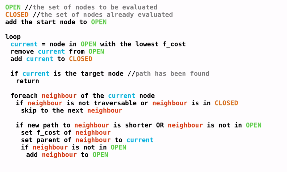
To start off with, we create two lists. The first is called the Open List. 08:00 And this list is for storing all of the
nodes for which we have already calculated the F cost. So in the diagrams I’ve been showing, all the nodes that were colored green were the ones that were currently in the open list, then the closed list is basically the set of nodes that have already been evaluated. Those were all of the ones I sort of ticked off as red in the diagrams, once we’d looked at all of their neighbors.
So once we’ve created those two lists, we add the starting node to the open list,

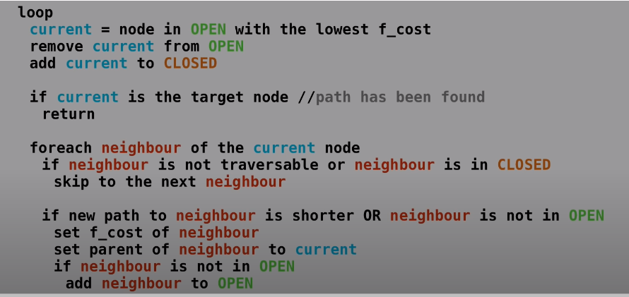
so that’s currently the only thing in the open list. And there’s nothing, of course, at the start in the closed list. And then we enter a loop. So inside of the loop we create a little temporary variable called our current node. And this is equal to the node in the open list with the lowest F cost. 08:50 So at the beginning, that will of course be the starting node since it’s the only one in the open list, and we remove the current node from the open list and we add it to the closed list. Then if the current node is the
target node, then we can assume that we found the path and we can just exit out of the loop.

Otherwise we’re going to go through each of the neighboring nodes of the current node.

And first of all, if it’s not traversable or if it’s in the closed list, then we’ll just skip ahead to the next neighbour and ignore it.

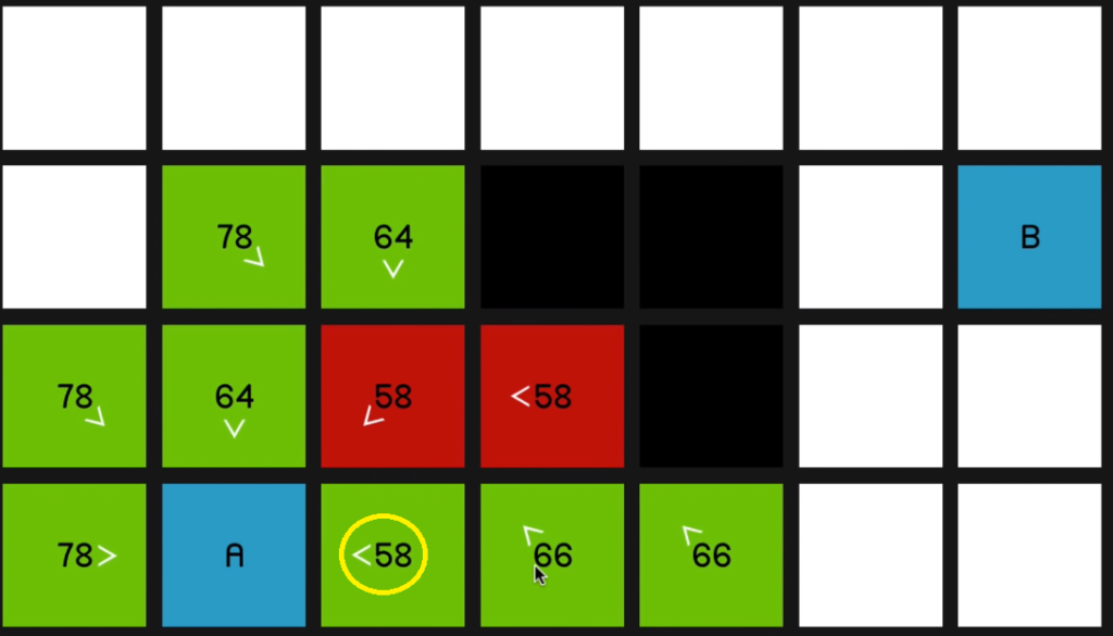
And if that’s not the case, then we check a couple of things. So first of all: if the new path to the
neighbor is shorter than the old path. So say, for example, that the neighbour is already in the open list, as we’ve seen in some of the diagrams, but then the new path is shorter.
So we have to update that node to reflect that we found a better path to it. (In this case the F=58)
09:51
So if if that is true or if the neighbour is not already in the open list,

then we set the F cost of the neighbour, which we do obviously by first calculating the G cost and the H cost,

and then we set the parent of the neighbour to the current node.

So that’s what I was sort of trying to show visually with the arrows:
we sort of keep a reference to where that node came from so that we can retrace the steps once we get to the end node.
Then finally, if the neighbor is not in the open list,

then we just add the 10:24 neighbour to the open list

and we keep looping this.
And eventually the current node is going to be equal to the target node and the path will have been found, and we’ll exit out of the loop. And we’ll just run a quick little method to look at all of the parents going back from the end node until we find the starting node. And that will be our path.